
✍️ 𝐁𝐲 𝐀𝐛𝐡𝐢𝐬𝐡𝐞𝐤 𝐊𝐮𝐦𝐚𝐫 | #𝐅𝐢𝐫𝐬𝐭𝐂𝐫𝐚𝐳𝐲𝐃𝐞𝐯𝐞𝐥𝐨𝐩𝐞𝐫
Ever wondered how AI can tell whether an image is a dog or something else?
Behind that simple “dog or not dog” prediction lies one of the most fascinating pieces of modern computer science — neural networks. These systems learn to see patterns in the same way humans do — by observing, comparing, and refining knowledge through feedback.
Let’s unpack the process layer by layer, and understand what’s really happening under the hood from a developer’s and architect’s point of view.
1. Training – Teaching the Neural Network to See
Training a neural network is like teaching a child how to recognize animals.
We feed the model thousands (or millions) of labeled images: dogs, cats, elephants, birds, etc. Each image is associated with a label, e.g., “dog.”
Technically:
- Each image is converted into a matrix of pixel values (for RGB, three matrices: Red, Green, Blue).
- The neural network starts with random weights — small numbers that represent how strongly one neuron’s output influences another.
- During training, the network predicts an output (say “cat”), compares it to the real label (“dog”), and calculates loss (the error).
- It then uses backpropagation and gradient descent to adjust the weights slightly, reducing the loss for the next iteration.
After thousands of iterations, the network learns the distinguishing patterns that define a “dog” — fur textures, ear shapes, nose patterns, etc.
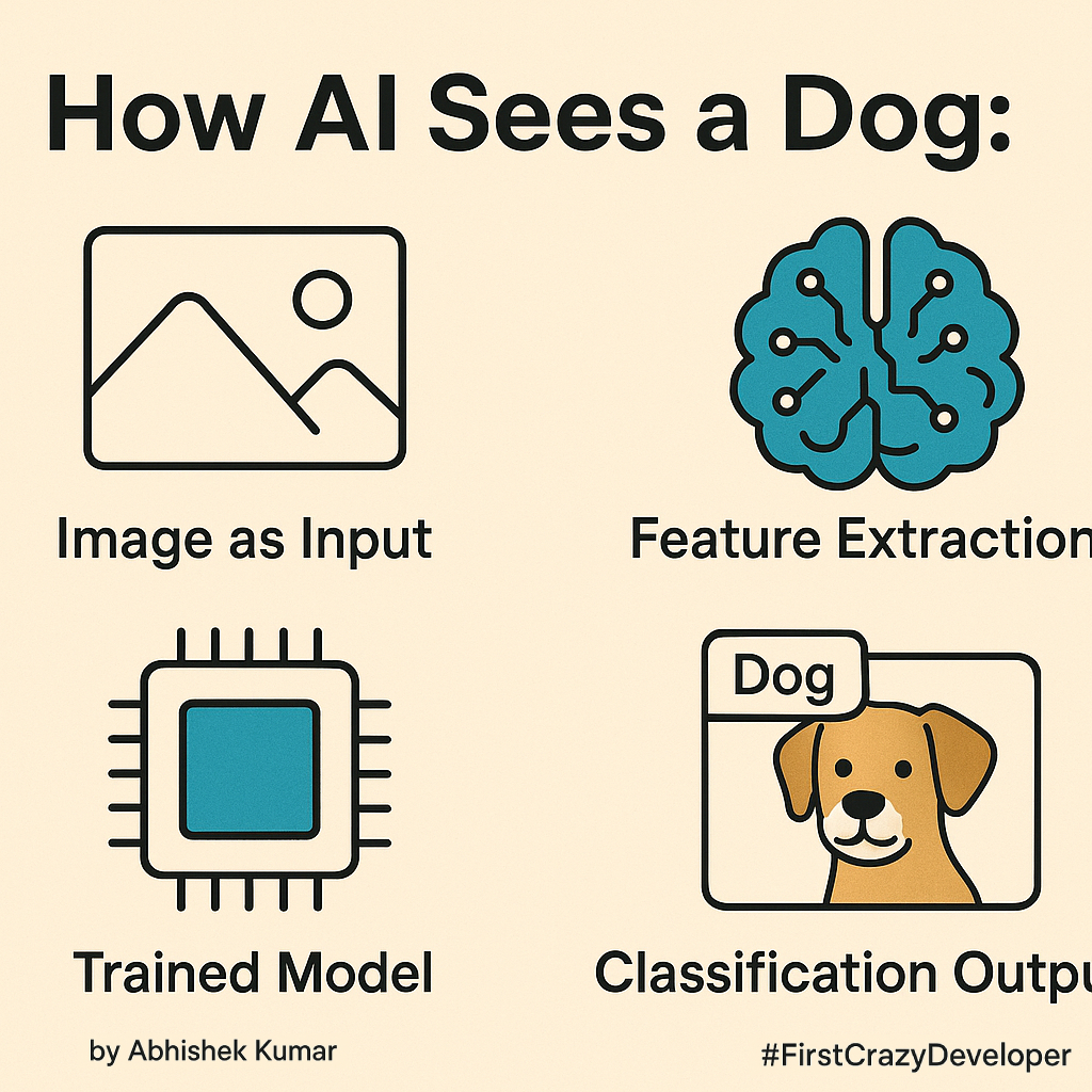
2. Input – A New Photo Arrives
Once trained, we present the model with a new, unlabeled image (a dog, but the model doesn’t know that).
This image passes through the trained layers, and each layer extracts increasingly meaningful information from it.
For example:
- Input: a 224×224×3 image (width, height, RGB channels)
- Output (at the end): probability scores like
[0.9 Dog, 0.1 Wolf]
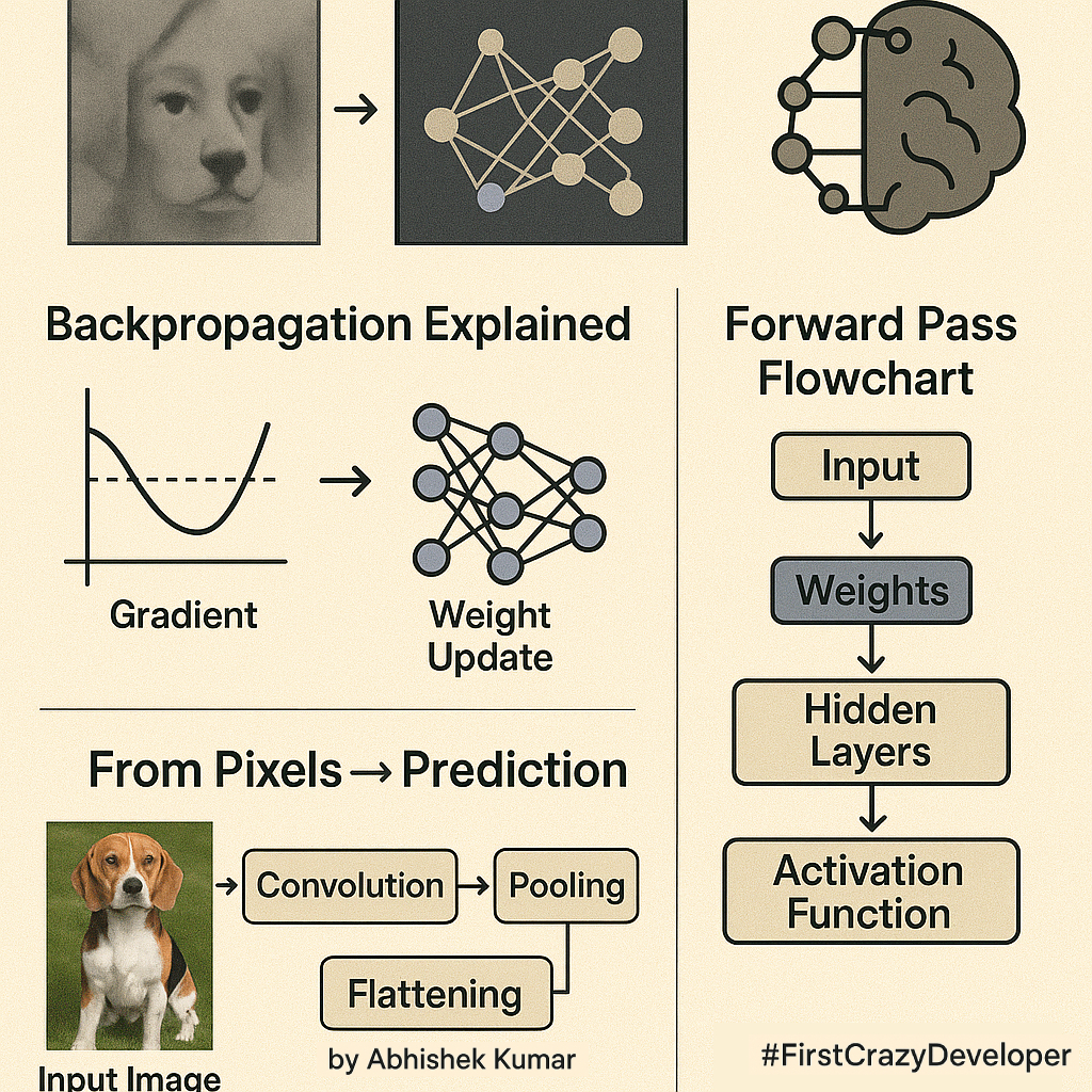
3. First Layer – Detecting Basic Features
The first layer (often a convolutional layer) identifies low-level features:
- Edges, corners, and simple textures.
- It applies filters or kernels — small matrices that slide over the image and compute convolutions (dot products of pixels and kernel values).
- These highlight local patterns like “a vertical line,” “a color gradient,” or “a fur-like texture.”
In essence, this layer builds a feature map showing where simple visual elements exist in the image.
4. Higher Layers – Recognizing Complex Patterns
As we move deeper:
- The second and third layers combine earlier features to detect parts of objects: curves, tails, eyes, ears.
- The network starts piecing together these local cues into a bigger semantic picture.
Technically, this is where non-linear activation functions (like ReLU) and pooling layers help:
- ReLU introduces non-linearity, allowing the network to model complex real-world shapes.
- Pooling reduces spatial size while keeping key features, improving computation and generalization.
By this stage, the network can tell: “There are four legs, a tail, and fur — this could be an animal.”
5. Top Layer – Decision Making
At the top of the network, we reach the fully connected layers (dense layers).
Here, all extracted features are combined and interpreted.
The final layers don’t look at raw pixels anymore — they analyze abstract feature vectors that summarize the entire image.
They compare these learned patterns to the ones seen during training:
“This combination of features — fur texture + snout shape + ear position — most closely matches the ‘dog’ class, not ‘cat’ or ‘wolf’.”
The network’s output layer (often a softmax layer) converts these raw scores into probabilities.
6. Output – The Final Prediction
Finally, the model outputs a probability distribution across all known classes:
- Dog: 0.90
- Wolf: 0.10
- Cat: 0.00
So it concludes:
“I’m 90% confident this is a dog and 10% it’s a wolf.”
7. Why It Works – Learning Through Error
The magic lies in continuous feedback:
- Every wrong prediction fine-tunes the weights through gradient descent.
- Over time, the model becomes extremely accurate at recognizing subtle patterns — even under different lighting, angles, or backgrounds.
This process is known as representation learning — the model automatically discovers the features that best represent the concept of “dog.”
8. Architectural Perspective
From an architect’s lens, here’s what the system looks like:
| Component | Description |
|---|---|
| Input Layer | Takes in raw image pixels |
| Convolution Layers | Extract spatial features using filters |
| Pooling Layers | Downsample feature maps to reduce dimensionality |
| Dense Layers | Combine and interpret features |
| Softmax Output Layer | Produces probability for each class |
| Loss Function | Measures prediction error |
| Optimizer (e.g., Adam, SGD) | Adjusts weights to minimize loss |
Frameworks like TensorFlow, PyTorch, or Keras make it easy to implement these components and visualize what the model is learning at each stage.
9. Beyond Dogs – Broader Applications
The same principle powers:
- Face Recognition (detecting eyes, nose, mouth, etc.)
- Medical Imaging (identifying tumors in scans)
- Autonomous Vehicles (recognizing pedestrians and road signs)
- Manufacturing (detecting product defects)
In each case, the network learns unique visual cues — from pixels to patterns to meaning.
🧠 Let’s go step by step and see how it works, both conceptually and in code using PyTorch.
⭐ Training – Teaching the AI What “Dog” Means
Before recognizing anything, a neural network must be trained.
We show it thousands of labeled pictures of animals — dogs, cats, elephants, etc.
It learns what makes each one unique by adjusting its internal parameters called weights.
What happens:
- Each image is turned into a 3D array (height × width × color channels).
- The model predicts a label (e.g., “cat”).
- The error between prediction and truth (called loss) is calculated.
- Using backpropagation, the model slightly adjusts its weights to reduce this error.
This process repeats thousands of times until the network gets very good at identifying dogs.
🖼️ Input – Giving a New Image
Once the model is trained, we feed it a new image — say, a dog photo.
from PIL import Image
from torchvision import transforms

# Load image
img = Image.open("dog.jpg")

# Convert to tensor and normalize
transform = transforms.Compose([
    transforms.Resize((224, 224)),
    transforms.ToTensor(),  # converts to [C,H,W] format
    transforms.Normalize(mean=[0.485, 0.456, 0.406],
                         std=[0.229, 0.224, 0.225])
])

input_image = transform(img).unsqueeze(0)  # Add batch dimension
The image is now just numbers — tensors the network can understand.
🔍 First Layer – Detecting Edges and Colors
The first layer is called a Convolution Layer.
It looks for basic patterns — edges, corners, and textures.
Concept:
Each convolutional filter slides across the image and highlights specific patterns like “horizontal edge” or “color contrast.”
import torch
import torch.nn as nn

# First convolution layer
conv1 = nn.Conv2d(in_channels=3, out_channels=8, kernel_size=3, stride=1, padding=1)

# Apply the layer
out1 = conv1(input_image)
print(out1.shape)  # e.g., torch.Size([1, 8, 224, 224])
Here, 8 filters scan the image to produce 8 feature maps — each showing where a certain pattern appears.
At this stage, the network doesn’t “see” a dog — it only sees lines, edges, and color gradients.
🧩 Higher Layers – Recognizing Shapes and Parts
As we move deeper, the network starts combining edges into shapes — curves, legs, ears, eyes, etc.
This happens through multiple convolution and pooling layers.
layer2 = nn.Sequential(
    nn.Conv2d(8, 16, kernel_size=3, stride=1, padding=1),
    nn.ReLU(),                # Adds non-linearity
    nn.MaxPool2d(kernel_size=2, stride=2)  # Downsamples the image
)

out2 = layer2(out1)
print(out2.shape)  # torch.Size([1, 16, 112, 112])
What’s happening:
ReLUhelps the model learn complex patterns by adding non-linear behavior.MaxPool2dreduces the image size, keeping only the most important information.
By now, the AI starts piecing together what it’s seeing — “four legs,” “fur,” “tail.”
🧠 Top Layers – Understanding the Whole Picture
At the top of the network, fully connected (dense) layers combine everything learned before.
They take all the detected features and try to identify which class (dog, cat, wolf, etc.) best matches.
# Flatten the output for the fully connected layer
flattened = out2.view(out2.size(0), -1)

fc = nn.Linear(flattened.shape[1], 3)  # Let's say 3 classes: dog, cat, wolf
output = fc(flattened)
print(output)
Now, the network outputs raw scores for each class, like:
tensor([[2.1, -0.5, 1.3]]) # Example: [dog, cat, wolf]
📊 Output – Making a Prediction
Finally, the model converts these scores into probabilities using a softmax function.
probabilities = torch.nn.functional.softmax(output, dim=1)
print(probabilities)
Example output:
tensor([[0.90, 0.05, 0.05]]) # 90% dog, 5% cat, 5% wolf
So, the AI confidently says:
“I’m 90% sure this is a dog and 10% it’s something else.”
🔄 How the AI Improves – Learning from Errors
When the network guesses wrong during training:
- It calculates loss (difference between guess and actual answer).
- It uses gradient descent to adjust weights.
- Each pass improves its accuracy slightly.
Example training snippet:
criterion = nn.CrossEntropyLoss()
optimizer = torch.optim.Adam(conv1.parameters(), lr=0.001)

# Dummy labels (dog = class 0)
labels = torch.tensor([0])

loss = criterion(output, labels)
loss.backward()      # Backpropagation
optimizer.step()     # Update weights
This process — repeated thousands of times — makes the model more accurate.
🧱 Putting It All Together
Here’s how a simple neural network might look when combined:
class DogClassifier(nn.Module):
    def __init__(self):
        super(DogClassifier, self).__init__()
        self.conv_layers = nn.Sequential(
            nn.Conv2d(3, 8, 3, 1, 1),
            nn.ReLU(),
            nn.MaxPool2d(2, 2),
            nn.Conv2d(8, 16, 3, 1, 1),
            nn.ReLU(),
            nn.MaxPool2d(2, 2)
        )
        self.fc = nn.Linear(16 * 56 * 56, 3)  # assuming input 224x224

    def forward(self, x):
        x = self.conv_layers(x)
        x = x.view(x.size(0), -1)
        x = self.fc(x)
        return torch.nn.functional.softmax(x, dim=1)

model = DogClassifier()
result = model(input_image)
print(result)
🌍 Beyond Dogs – Real-World Uses
This same concept powers many AI systems:
- Face Recognition – detecting eyes, nose, mouth patterns.
- Medical Imaging – identifying tumors.
- Autonomous Cars – detecting people, roads, and signs.
- Quality Control – spotting defects in manufacturing.
Wherever pattern recognition is needed, convolutional neural networks (CNNs) are the foundation.
💡 Final Thoughts
Neural networks don’t “see” like humans — they mathematically model perception.
But the idea is the same: from observing thousands of examples, they learn what features define an object, and how to tell it apart from others.
Neural networks analyze patterns of numbers.
But through layers of training, they learn:
- First: basic shapes
- Then: object parts
- Finally: meaning
Every layer adds understanding — from edges → shapes → features → recognition.
So when your AI says, “This is a dog,” it’s not guessing — it’s the result of thousands of learned visual patterns, all working together.
Every layer transforms raw data into deeper understanding — from edges → patterns → shapes → meaning — until finally, the network can look at a photo and say with confidence:
“That’s a dog.”
In short: Neural networks learn to recognize by seeing, comparing, and adjusting — until they can confidently tell what’s in a photo.
It’s not magic, it’s mathematical learning at scale.
#AI #DeepLearning #NeuralNetworks #MachineLearning #ComputerVision #ArtificialIntelligence #Developers #TechBlog #LearningAI #FirstCrazyDeveloper #AbhishekKumar

Leave a comment